Linear Layouts in Triton
Published:
This post is temporarily written in Chinese for convenience. It may be converted to an English version later. If you prefer reading in English, you may use the default translation feature of your browser. Sorry for the inconvenience!
本帖暂时用中文写,稍微方便点。后面有可能会转换为英文版。
Linear Layouts
Concepts
In Triton, a linear layout (LL) is a function that maps from a “hardware location” to a “logical tensor index”.
简而言之,linear layout 是一个函数 $\mathcal{L}$,将硬件资源的布局映射到对应的 logical tensor 坐标上。其之所以被称为线性的(linear),是在以下两个意义上线性:
硬件资源的布局和 logical tensor 的坐标都可以使用二进制数来表示。这得益于硬件资源(如 registers、threads、warps、CTA blocks 等)和 logical tensor 坐标的各个维度通常都是 2 的幂次。
layout 函数在异或(xor,通常记为⊕)运算下是线性的。由于硬件坐标和 logical tensor 坐标都可以用二进制数表示,xor 运算可以被视为对二进制数的每一位进行独立的无进位加法运算: \(0\oplus0=0,\ 0\oplus1=1,\ 1\oplus0=1,\ 1\oplus1=0\)
使用 xor 运算(而不是通常的加法运算)来描述线性性质,看起来有些难以理解。其一大好处是可以用来描述 swizzling(混洗)操作。Triton Linear Layout: Concept 一文中提到的第二个例子就是 swizzling layout 的一个例子,其中便使用了 xor 操作。1
有了以上概念,linear layout $\mathcal{L}$ 的线性性质可以用数学语言描述为:
\[\mathcal{L}(x_0\oplus y_0, x_1\oplus y_1, \cdots, x_n\oplus y_n) = \mathcal{L}(x_0, x_1, \cdots, x_n) \oplus \mathcal{L}(y_0, y_1, \cdots, y_n)\]由于 linear layout 的每个输入坐标 $x_i$ 都是二进制数,我们可以自然地把多维坐标 $(x_0, x_1, \cdots, x_n)$ 前后连接到一起展平成一维,形成一个更长的二进制数。因此,所有的 linear layout 都可以被视为一个一维的函数 $\mathcal{L}(x=b_0b_1…b_n)$,其中 $b_i$ 是二进制数的每一位。
对于满足上述线性性质的 linear layout $\mathcal{L}$,我们只需要部分的输入输出坐标对 $x_k \mapsto y_k$,就可以利用线性性质求出任意的输入输出坐标对。最简单也是最自然的输入坐标即为 2 的幂次的整数 $x_k = 2^k=(00…010…0)_2$。由于 xor 运算是无进位加法,任意输入坐标 $x_k$ 都可以被表示为若干个 2 的幂次的整数的异或和,相应的输出坐标 $y_k$ 也可以被表示为若干个输出坐标的异或和。以下面例子为例,输入坐标 $(t, w)$ 均在 $[0, 3]$ 范围内,给出了 $(0, 1)$、$(0, 2)$、$(1, 0)$ 和 $(2, 0)$ 四个输入坐标的输出坐标:
\[\begin{align*} \mathcal{L} (0, 1) = (0, 1) \\ \mathcal{L} (0, 2) = (0, 2) \\ \mathcal{L} (1, 0) = (1, 1) \\ \mathcal{L} (2, 0) = (2, 2) \\ \end{align*}\]任意输入坐标 $(t, w)$ 都可以表示为 $t = 2^0 \cdot t_0 \oplus 2^1 \cdot t_1$ 和 $w = 2^0 \cdot w_0 \oplus 2^1 \cdot w_1$,其中 $t_i, w_i \in {0, 1}$。这样,我们就能计算出任意输入坐标对应的输出坐标:
\[\begin{align*} \mathcal{L} (1, 3) &= \mathcal{L} (1, 0) \oplus \mathcal{L} (0, 1) \oplus \mathcal{L} (0, 2) \\&= (1, 1) \oplus (0, 1) \oplus (0, 2) = (1, 2) \end{align*}\]因此,我们可以把 $(0, 1)$、$(0, 2)$、$(1, 0)$ 和 $(2, 0)$ 四个输入坐标看成是 linear layout 的基向量(basis vectors),他们都对应 2 的幂次的整数。
Triton 里最基本的 linear layout 有两个:identity layout 和 zero layout。
LinearLayout::identity1D:将 $[0, \text{size})$ 范围内的整数进行恒等映射 $\mathcal{L}(x) = x$。static LinearLayout identity1D(int32_t size, StringAttr inDim, StringAttr outDim);LinearLayout::zeros1D:将 $[0, \text{size})$ 范围内的整数映射为 0,即 $\mathcal{L}(x) = 0$。static LinearLayout zeros1D(int32_t size, StringAttr inDim, StringAttr outDim);
这两种最基本的 linear layout 可以通过乘法构造出更复杂的 linear layout。除此以外,Triton 提供了方便的 constructor 来构造 linear layout。
LinearLayout(BasesT, ArrayRef<StringAttr>):通过一组完备的基向量输入输出对来构造 linear layout。这种构造会自动检查该 linear layout 是否为满射(surjective),即是否能覆盖所有的 logical tensor 坐标。
#include "mlir/IR/MLIRContext.h"
#include "llvm/ADT/MapVector.h"
#include "LinearLayout.h"

// Setup necessary MLIR components
mlir::MLIRContext context;
auto inDim1 = mlir::StringAttr::get(&context, "in1");
auto outDim1 = mlir::StringAttr::get(&context, "out1");
auto outDim2 = mlir::StringAttr::get(&context, "out2");

// Create a layout by defining the bases directly.
using BasesT = llvm::MapVector<mlir::StringAttr,
                            std::vector<std::vector<int32_t>>>;
BasesT bases;
bases[inDim1] = {
    {1, 0}, // L(in1=1) = (out1=1, out2=0)
    {5, 1}, // L(in1=2) = (out1=5, out2=1)
    {2, 2}  // L(in1=4) = (out1=2, out2=2)
};

std::vector<mlir::StringAttr> outDimNames = {outDim1, outDim2};

// This constructor infers output sizes and requires the map to be surjective.
LinearLayout layout(bases, outDimNames);

// layout.getOutDimSize("out1") would be 8 (next power of 2 >= 5)
// layout.getOutDimSize("out2") would be 4 (next power of 2 >= 2)
- 可以使用 C++ initializer lists ({…}) 来简化初始化:
#include "mlir/IR/MLIRContext.h"
#include "LinearLayout.h"

// Setup
mlir::MLIRContext context;
auto in1 = mlir::StringAttr::get(&context, "in1");
auto in2 = mlir::StringAttr::get(&context, "in2");
auto out1 = mlir::StringAttr::get(&context, "out1");
auto out2 = mlir::StringAttr::get(&context, "out2");

// Use the initializer-list friendly constructor.
LinearLayout layout(
    /* bases */
    {
        {in1, { {0, 1}, {0, 2}}}, // L(in1=1)={0,1}, L(in1=2)={0,2}
        {in2, { {0, 4}, {0, 8}, {1, 1}}} // L(in2=1)={0,4}, L(in2=2)={0,8}, L(in2=4)={1,1}
    },
    /* outDimNames */
    {out1, out2}
);
LinearLayout(BasesT, ArrayRef<pair<StringAttr, int32_t>>, bool):同样通过一组完备的基向量输入输出对来构造 linear layout,并且可以选择是否检查该 linear layout 是否为满射。由于非满射情况下无法自动推断出输出维度的大小,因此需要手动指定输出维度的大小。
#include "mlir/IR/MLIRContext.h"
#include "llvm/ADT/MapVector.h"
#include "LinearLayout.h"

// Setup necessary MLIR components
mlir::MLIRContext context;
auto inDim1 = mlir::StringAttr::get(&context, "in1");
auto outDim1 = mlir::StringAttr::get(&context, "out1");

// Create a non-surjective layout with explicit output sizes.
using BasesT = llvm::MapVector<mlir::StringAttr,
                              std::vector<std::vector<int32_t>>>;
BasesT bases;
bases[inDim1] = {
    {1}, // L(in1=1) = (out1=1)
    {4}  // L(in1=2) = (out1=4)
};

// Explicitly define the output dimension and its size.
std::vector<std::pair<mlir::StringAttr, int32_t>> outDims = {
    {outDim1, 32} // The codomain for out1 is [0, 32), even though we only
                  // produce values up to 5.
};

// Create the layout, specifying that it doesn't need to be surjective.
LinearLayout layout(bases, outDims, /*requireSurjective=*/false);
- 同样,可以使用 C++ initializer lists ({…}) 来简化初始化:
#include "mlir/IR/MLIRContext.h"
#include "LinearLayout.h"

// Setup
mlir::MLIRContext context;
auto inDim1 = mlir::StringAttr::get(&context, "in1");
auto outDim1 = mlir::StringAttr::get(&context, "out1");

//  Use the initializer-list friendly constructor for a non-surjective layout.
LinearLayout layout(
    /* bases */
    {
        {inDim1, { {1}, {4}}} // L(in1=1) = {1}, L(in1=2) = {4}
    },
    /* outDims */
    {
        {outDim1, 32} // Explicitly specify size of out1 is 32.
    },
    /* requireSurjective */
    false
);
Multiplication
两个 linear layout 可以通过乘法构造出新的 linear layout。在讲解乘法之前,我们应当强调,linear layout 的输入和输出坐标是命名的,从上面给的几个例子里也能看出这一点。对于单独的一个 layout,输入和输出的名称是任意的,只是为了表示有不同输入和输出的通道;但是,在两个 linear layout 相乘时,他们可以有相同的输入/输出名称,也可以是不同的——相同的输入/输出名称表示两个 linear layout 使用相同的输入/输出通道。我们下面分情况进行讨论。
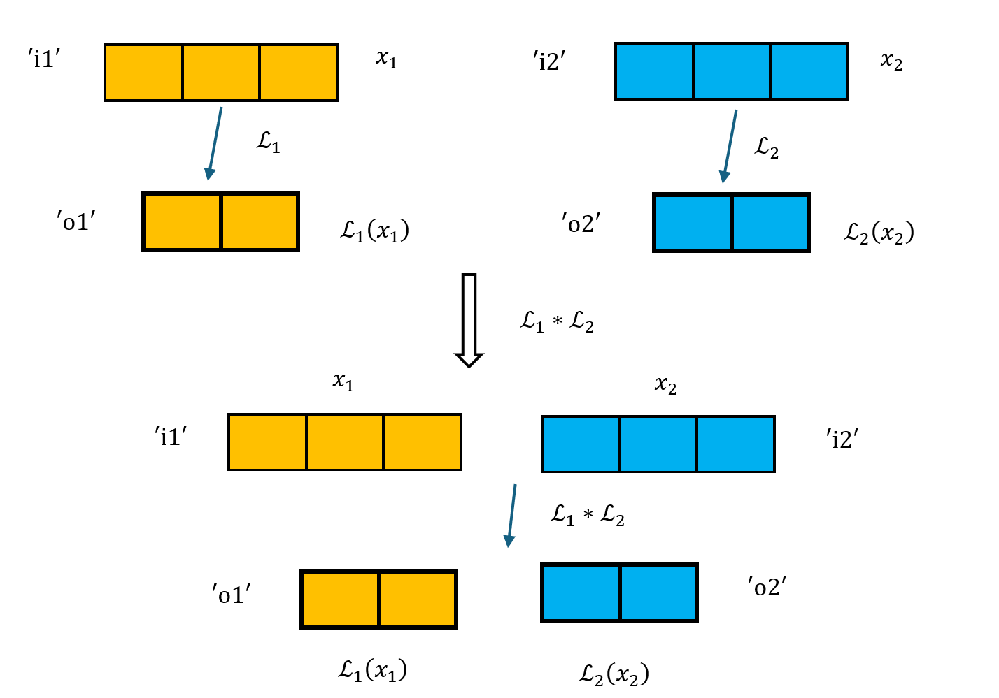
输入和输出的名称均不重合:直接将两个 linear layout 的输入输出坐标进行拼接。
\[\begin{align*} &\mathcal{L}_1(x_1; \text{`i1'}; \text{`o1'}) * \mathcal{L}_2(x_2; \text{`i2'}; \text{`o2'})\mapsto \mathcal{L}(x_1, x_2; \text{`i1'}, \text{`i2'}; \text{`o1'}, \text{`o2'}) \\ &\text{such that } \mathcal{L}(x_1, x_2) = (\mathcal{L}_1(x_1), \mathcal{L}_2(x_2)) \end{align*}\]如下图所示,图示中所有的方格代表二进制表示的一个 bit,$\mathcal{L}_1$ 和 $\mathcal{L}_2$ 的输入输出坐标分别用不同的颜色表示。可以看到,$\mathcal{L}_1 * \mathcal{L}_2$ 的输入输出坐标仅仅只是 $\mathcal{L}_1$ 和 $\mathcal{L}_2$ 的输入输出坐标的拼接。
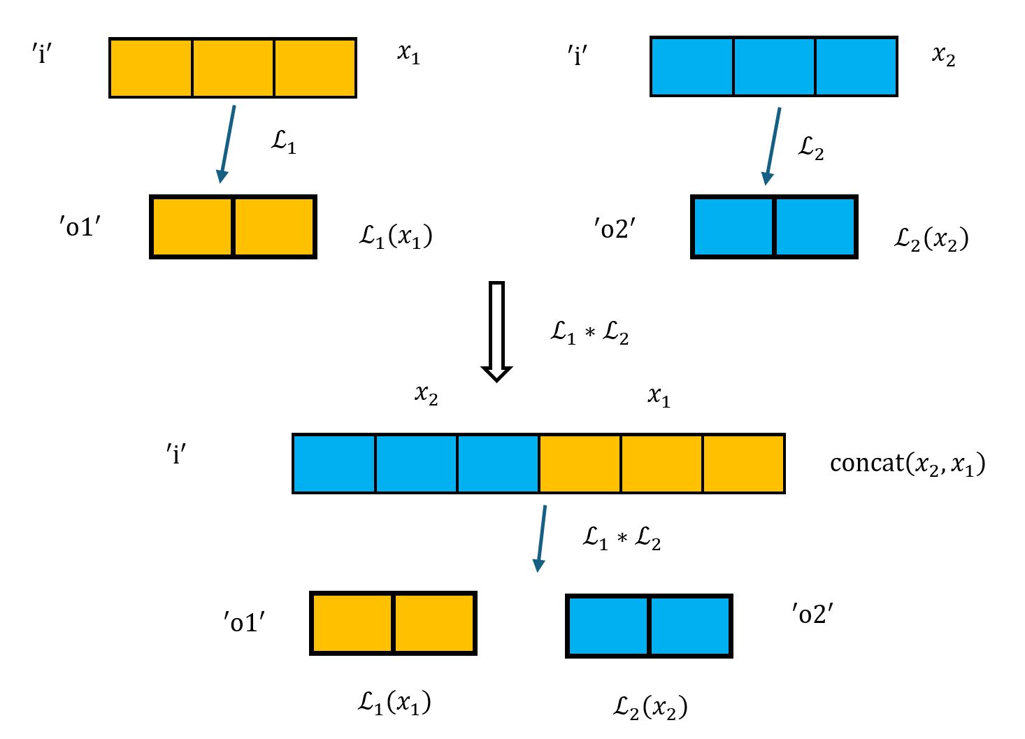
输入的名称重合,输出的名称不重合:合成的 layout 将输入合成为一个通道,将输出拼接。
\[\begin{align*} &\mathcal{L}_1(x_1; \text{`i'}; \text{`o1'}) * \mathcal{L}_2(x_2; \text{`i'}; \text{`o2'})\mapsto \mathcal{L}(x; \text{`i'}; \text{`o1'}, \text{`o2'}) \\ &\text{such that } \mathcal{L}(x) = (\mathcal{L}_1(x_1), \mathcal{L}_2(x_2)), \text{ where } x = \text{concat}(x_2, x_1) \end{align*}\]如下图所示,将输入合成为一个通道时,乘号前 layout($\mathcal{L}_1$)的输入放在低位,乘号后 layout($\mathcal{L}_2$)的输入放在高位。
除此以外,还有两种可能的情况,分别是输出名称重合、输入输出名称均重合。合成通道和拼接的规则和上面完全相同,在此不再赘述。
- 输入的名称不重合,输出的名称重合:合成的 layout 将输出合成为一个通道,将输入拼接。
- 输入输出的名称均重合:合成的 layout 将输入输出均合成为一个通道。
有了以上定义的乘法规则,我们就可以用最基本的 identity1D 和 zeros1D 来构造出更复杂的 linear layout。我们可以看几个例子。
$\mathcal{L}(x) = x / 4$,$x \in [0, 8)$;该 layout 可视作
zeros1D(4, "i", "o") * identity1D(2, "i", "o"),因其等效于直接舍弃 $x$ 的低两位。$\mathcal{L}(x) = x \text{ \% } 4$,$x \in [0, 8)$;该 layout 可视作
identity1D(4, "i", "o") * zeros1D(2, "i", "o"),因其等效于直接舍弃 $x$ 的最高位。$\mathcal{L}(x) = (x \text{ \% } 4,\ x / 4)$,$x \in [0, 32)$;该 layout 可视作
identity1D(4, "i", "o1") * identity1D(8, "i", "o2"),因其等效于直接将 $x$ 的低两位和高三位分别作为两个输出。
Convertion to Traditional Layouts
CTA Layouts
硬件(GPU)最小的计算单元是 thread,每个 thread 有若干 registers 用来存储数据,各个 thread 之间可以并行运算。一个 warp 由若干 threads 组成,通常是 32 个。一个 CTA block 由若干 warps 组成。最后,一个 CGA block 由若干 CTA blocks 组成,完成一个完整的计算任务。通常而言,这些组成的倍数都是 2 的幂次。
以矩阵乘法为例,假设有两个矩阵 $A$ 和 $B$,大小分别是 $M \times K$ 和 $K \times N$,现在想要计算矩阵 $C = AB$。每对元素的乘法 $a_{ij} \cdot b_{jk}$ 由一个 thread 来完成;一整行与一整列之间的乘法 $c_{ik}=\sum_{j}a_{ij} \cdot b_{jk}$ 由一个或多个 warp 来完成;一个 CTA block 则负责计算 $C$ 的一块小区域;最后,一个 CGA block 通过若干 CTA blocks 来计算整个矩阵 $C$。
CTA layout 的目的是将硬件资源的布局映射到对应的 logical tensor 坐标上;比如,这块 CTA block 负责 logical tensor 的哪一块数据,或者这个 register 存储了 logical tensor 的哪个元素。根据文档(LinearLayoutConversions.cpp)里的定义,我们可以将 CTA layout 按照层次的不同分为两类:
- cgaLayout:一块 CGA block 被划分为若干 CTA blocks,相应地,所对应的 logical tensor 也被划分为若干 blocks。该 layout 将 CTA block 的坐标映射到 logical tensor 的 block 坐标上。
- ctaLayout:一块 CTA block 内部有许多 warps,每个 warp 内部有许多 threads,每个 thread 内部有若干 registers。该 layout 将(warp_index, thread_index, register_index)映射到对应的 logical tensor block 内部的相对坐标上。
文档同时指出,不同文档的命名法多有混淆和差别。比如,该文档(TritonGPUAttrDefs.td)中定义的 CTALayoutAttr 实际上是我们这里的 cgaLayout。
cgaLayout (CTALayoutAttr)
声明一个 cgaLayout 需要指定以下参数:
CTAsPerCGA:每个 CGA block 是如何分割为若干 CTA blocks 的。比如,CTAsPerCGA = [2, 4]表示每个 CGA block 被分割为 2x4 个 CTA blocks。CTASplitNum:logical tensor 是如何分割为若干 blocks 的。比如,CTASplitNum = [2, 4]表示 logical tensor 被分割为 2x4 个 blocks。CTAOrder:对于多维的 CTA blocks,当展平为一维时的排列顺序。比如,CTAOrder = [1, 0]表示先按 dim1(一整行从左到右)排列,再按 dim0(再从上到下)排列。
多个 CTA block 可以对应同一块 logical tensor block。比如,如果 CTAsPerCGA[0] = 8,CTASplitNum[0] = 2,则 CTA 在第 0 个维度上被分成 8 份,交替映射到 logical tensor 被分成的 2 份上,分配的方式为 (0, 1, 0, 1, 0, 1, 0, 1)。从这个例子也可以看出,CTAsPerCGA 和 CTASplitNum 的每个维度上的值必须是整数倍数关系。在转换为 linear layout 时,函数将默认检查上述条件。在该条件满足时,cgaLayout 的数学表达式可以写为:
其中,$(x_0, x_1, \cdots, x_n)$ 是 CTA block 的坐标,坐标限定在 CTAsPerCGA 给定的范围内;$\text{split}[i]$ 是 CTASplitNum 在第 $i$ 个维度上的值。
如果每个维度上的 CTAsPerCGA 和 CTASplitNum 都是 2 的幂次,则可以将 cgaLayout 转换为 linear layout。这时,cgaLayout 的输入坐标 $(x_0, x_1, \cdots, x_n)$ 每一个都可以用二进制来表示,再按照 CTAOrder 给出的顺序从低位到高位排列。比如,如果 CTAsPerCGA = [2, 4],CTASplitNum = [2, 4],CTAOrder = [1, 0],则输入坐标 $(x_0, x_1)$ 可以分别表示为一个 1-bit 和一个 2-bit 的二进制数 $(b_0, b_1)$;再按照 CTAOrder 的顺序排列,得到的 linear layout 输入坐标为 $b_0b_1$,即 $b_1$ 在低位,$b_0$ 在高位。坐标 $(1, 1)$ 按照上述规则转换为 linear layout 输入坐标为 $b_0b_1 = (101)_2$。同时,为了能够表示取余操作,我们可以利用 layout 的乘法(参见上文),将 $x \text{ \% } a$ 转换为 identity1D(a, "i", "o") * zeros1D(size/a, "i", "o")。具体 makeCgaLayout(layout) 实现的代码梗概如下:
// makeCgaLayout
// (CTALayoutAttr layout)
LinearLayout ret = LinearLayout::empty(); // Initialization
for (int i = 0; i < rank; i++) {
  // Start with the most minor dimension, which is order[0].
  // Check the divisibility condition
  int dim = layout.getCTAOrder()[i];
  int split = layout.getCTASplitNum()[dim];
  int ctas = layout.getCTAsPerCGA()[dim];
  assert(ctas % split == 0);
  // Create the linear layout for this dimension
  ret *= LinearLayout::identity1D(split, kBlock, outDimNames[dim]) *
         LinearLayout::zeros1D(ctas / split, kBlock, outDimNames[dim]);
}
// Transpose to standard order (dim0, dim1, ...).
return ret.transposeOuts(outDimNames);
ctaLayout
一般的 ctaLayout 会用 blocked layout 的方式来实现,具体请见 Blocked Layouts 一节。有了 ctaLayout 后,将 ctaLayout 和 cgaLayout 结合的方法相当简单:直接利用 layout 的相乘即可。(注:实际 blocked layout 的实现是已经将 ctaLayout 和 cgaLayout 结合在一起了,因此以下函数无需单独调用,它是 blocked layout 转换为 linear layout 过程中的一个辅助函数。)
// combineCtaCgaWithShape
// (LinearLayout ctaLayout, CTALayoutAttr cgaLayoutAttr, ArrayRef<int64_t> shape)
LinearLayout cgaLayout = makeCgaLayout(cgaLayoutAttr);
LinearLayout ret = (ctaLayout * cgaLayout).transposeOuts(outDimNames);
Shared Layouts
将一个给定的 logical tensor 依次按行存入 shared memory 时,为了避免所谓的 bank conflicts,通常会在直接存入数据之前先进行 swizzling(混洗)操作。我们下面详细讨论这一点。本节中讨论所使用的部分例子来自于 Triton Linear Layout: Concept 一文1。
一般而言,shared memory 会根据存储地址划分为若干个 bank,通常为 32 个。存储地址和其对应的 bank 之间转换关系为
\[\text{bank} = (\text{address} / 4) \text{ \% } \text{num\_banks}\]当各个 thread 读写或存入数据时,如果访问的地址分属于不同的 bank,则可以并行进行;然而,如果多个 thread 同时访问处在同一 bank 内的若干地址,这些 thread 必须依次序列式进行访问。这就是所谓的 bank conflicts。
假设我们现在需要处理一个 $16\times 32$ 的 logical tensor $A$。当读取数据时,如果不做任何的 swizzling 操作,$A$ 的每一行 32 个元素将被依次存入 shared memory 的 32 个 bank 中,如下图所示。假如现在需要读取 $A$ 的第 0 列所有元素(例如,想要求出 $A$ 的转置矩阵),观察下图可知,$A$ 的第 0 列所有元素均在 bank 0 中,因此需要依次读取 16 次才能完成读取操作,这显然是低效的。

如果我们能在存入数据时对其进行 swizzling 操作,我们有望避免上面的 bank conflicts。swizzling 操作的核心思想是将每一行的元素打乱顺序。一种常见的 swizzling 操作是利用 xor 运算,将第 $i$ 行的第 $j$ 个元素存入 shared memory 的第 $ i \oplus j$ 个 bank 中,如下图所示。第 0 行和原先存储方式相同,第 1 行交换了奇偶元素,第 2 行对间隔为 2 的两个元素进行交换,依此类推。这样,观察下图可知,$A$ 的第 0 列所有元素均分布在不同的 bank 中,因此可以并行读取 16 次完成读取操作。

用来描述 shared memory 中具体是如何 swizzle 的 layout 就是 SwizzledSharedLayout,它将 logical tensor 的 index(按照 order 给出的顺序,见下)映射到 swizzle 后的行、列坐标上。这里,我们先假设讨论的 logical tensor 都是 2 维的。对第 $i$ 行的 swizzle 操作可以一般性地表示为:
其中,$f(i)$ 由 layout 决定,我们下面称其为 phase;在上面的例子里,$f(i)=i$。声明一个 SwizzledSharedLayout 需要指定以下参数:
vec:进行 swizzle 时配对的数目。比如,vec = 2表示将相邻的两个元素配对视作一个元素,再进行 swizzle 操作。上面的例子里,vec = 1。perPhase:swizzle 操作的周期。比如,perPhase = 4表示每 4 行将 swizzle 的 phase 加一。上面的例子里,perPhase = 1。maxPhase:swizzle 操作的最大 phase(不包含)。比如,maxPhase = 4表示 swizzle 的最大 phase 为 4,到达之后置零重新开始。order:logical tensor index 排列的顺序,同时也决定 swizzle 操作对应的维度。比如,order = [1, 0]表示 index 按行优先顺序排列。对于高于 2 维的 logical tensor,swizzle 对order给出的头两个维度进行操作。如无特别说明,下面讨论的 logical tensor 均为 2 维且采用order = [1, 0]的顺序;其余的order和更高的维度只需要交换行列顺序即可。
下面展示了一些具体的 SwizzledSharedLayout 的例子,假设 shape=[4, 8] 。
vec=1, perPhase=2, maxPhase=2, order=[1,0]
[ 0,  1,  2,  3],  // phase 0 (xor with 0)
[ 4,  5,  6,  7],  // phase 0
[ 9,  8, 11, 10],  // phase 1 (xor with 1)
[13, 12, 15, 14],  // phase 1
[16, 17, 18, 19],  // phase 0
[20, 21, 22, 23],  // phase 0
[25, 24, 27, 26],  // phase 1
[29, 28, 31, 30]   // phase 1
vec=2, perPhase=1, maxPhase=4, order=[1,0]
[ 0,  1,  2,  3,  4,  5,  6,  7],
[10, 11,  8,  9, 14, 15, 12, 13],
[20, 21, 22, 23, 16, 17, 18, 19],
[30, 31, 28, 29, 26, 27, 24, 25]
从以上例子我们可以归纳出 SwizzledSharedLayout 的一般性数学形式。使用给出的参数,第 $i$ 行的 phase 可以表示为:
为了将该 SwizzledSharedLayout 转换为 linear layout,还需要指明进行 swizzle 操作的 shape。假设 swizzle 操作的 shape 为 $[M, N]$,则 swizzle 后 index 为 $k$ 的 logical tensor 将位于第 $i$ 行第 $j$ 列,满足:
上述关系的反变换式为:
\[\begin{align*} i &= \left\lfloor \frac{k}{N} \right\rfloor \\ j &= (k \text{ \% } N) \text{ \% vec} + \left(\left\lfloor \frac{k \text{ \% } N}{\text{vec}} \right\rfloor \oplus f(i) \right) \cdot \text{vec} \\ \end{align*}\]可以证明,当 shape $[M, N]$ 中的 $M$、$N$ 和 SwizzledSharedLayout 的各参数都是 2 的幂次时,上述 layout $\mathcal{L}(k) = (i, j)$ 满足线性性质。这是因为向下取整除法、取模和乘法运算在除数和乘数是 2 的幂次时都等价于提取二进制数的某些位,这样的操作自然是线性的。
直接使用上面的公式来构建 layout 当然可行,但未免过于复杂。由于已知该 layout 是线性的,我们可以直接获取所需的 basis vectors 输入输出对来构造 linear layout。将 SwizzledSharedLayout 转换为 linear layout 的代码梗概如下:
// swizzledSharedToLinearLayout
// (ArrayRef<int64_t> shape, SwizzledSharedEncodingAttr shared)
int colDim = shared.getOrder()[0];
int rowDim = shared.getOrder()[1];
int numCols = shape[colDim];
int numRows = shape[rowDim];

// Using basis vectors to construct the linear layout
std::vector<std::vector<int>> bases2D;
for (int logCol = 0; logCol < llvm::Log2_32(numCols); logCol++) {
  bases2D.push_back({0, 1 << logCol});
}
for (int logRow = 0; logRow < llvm::Log2_32(numRows); logRow++) {
  int row = 1 << logRow;
  int vec = shared.getVec();
  int perPhase = shared.getPerPhase();
  int maxPhase = shared.getMaxPhase();
  bases2D.push_back({row, (vec * ((row / perPhase) % maxPhase)) % numCols});
}
LinearLayout ctaLayout =
    LinearLayout({ {S("offset"), bases2D}}, {rowDimName, colDimName});

// Add the remaining dimensions
for (int i = 2; i < rank; i++) {
  int dim = shared.getOrder()[i];
  ctaLayout *=
      LinearLayout::identity1D(shape[dim], S("offset"), outDimNames[dim]);
}
除此以外,SharedLayout 还有许多变种,比如 NVMMASharedEncoding 和 AMDRotatingSharedEncoding。
Distributed Layouts
以下所描述的 Distributed Layout 是指 TritonGPUAttrDefs.td 文档中定义的 DistributedEncodingTrait 和 DistributedEncoding。
DistributedEncodingTrait 描述了最基本的行/列优先 layout。与前面介绍的 layout 类似,行/列等的优先顺序由 order 参数给出;比如,order = [1, 0] 表示行优先顺序(即 layout 对应的 index 沿着一行从左至右增加,一行结束后再开始下一行),order = [0, 1] 表示列优先顺序(即 layout 对应的 index 沿着一列从上至下增加,一列结束后再开始下一列)。除此以外,给出 layout 的 shape 即可。
shape = [4, 4], order = [0, 1]
-> layout = [0  4  8  12]
            [1  5  9  13]
            [2  6  10 14]
            [3  7  11 15]
DistributedEncoding 描述的则是 logical tensor(以下称作 $T$)分布到多个 thread 上的方式。声明一个 DistributedEncoding 只需要一个给定的 DistributedEncodingTrait,也即上方例子里的 layout 矩阵(以下称作 $L$)。文档里指出,$L$ 不需要和 $T$ 的 shape 一致,甚至不需要有相同的 rank,但为了方便,以下的讨论始终假设 $L$ 和 $T$ 的 rank 相同。记维度 $i$ 上 $L$ 和 $T$ 的长度分别为 $L.\text{shape}[i]$ 和 $T.\text{shape}[i]$。
- 当 $L.\text{shape}[i] > T.\text{shape}[i]$,即 logical tensor 在第 $i$ 个维度的长度长于 layout 矩阵时,该 tensor $T$ 在该维度上的每个元素将对应多个 thread:该维度第 $k$ 个元素分布到 $L[k]$,$L[k + T.\text{shape}[i]]$,$L[k + 2 \cdot T.\text{shape}[i]]$,$\cdots$ 所决定的这些 threads 上,其中 $k \in [0, T.\text{shape}[i])$。这被称作 broadcasting。
- 当 $L.\text{shape}[i] < T.\text{shape}[i]$,即 logical tensor 在第 $i$ 个维度的长度短于 layout 矩阵时,该 tensor $T$ 在该维度上的元素所对应的 thread 将呈现周期性分布:该维度第 $k$ 个元素分布到 $L[k \text{ \% } L.\text{shape}[i]]$ 所决定的 thread 上,其中 $k \in [0, T.\text{shape}[i])$。这被称作 wrapping around。
上面规则稍显抽象,下面通过一个例子来说明。假设 logical tensor $T$ 的 shape 为 $[2, 8]$,layout 矩阵 $L$ 的 shape 为 $[4, 4]$:
L = [0  1  2  3 ]
    [4  5  6  7 ]
    [8  9  10 11]
    [12 13 14 15]
- 在第 0 个维度(行)上,$L.\text{shape}[0] = 4 > T.\text{shape}[0] = 2$,因此 $T$ 在该维度上的每个元素将对应多个 thread。具体地,第 0 行的元素 $T[0, 0]$ 将分布到 $L[0, 0]$ 和 $L[2, 0]$ 所决定的两个 threads 上;第 1 行的元素 $T[1, 0]$ 将分布到 $L[1, 0]$ 和 $L[3, 0]$ 所决定的两个 threads 上,依此类推。
- 在第 1 个维度(列)上,$L.\text{shape}[1] = 4 < T.\text{shape}[1] = 8$,因此 $T$ 在该维度上的元素所对应的 thread 将呈现周期性分布。具体地,第 0 列的元素 $T[0, 0]$ 和第 4 列的元素 $T[0, 4]$ 对应的 threads 相同;第 1 列的元素 $T[0, 1]$ 和第 5 列的元素 $T[0, 5]$ 对应的 threads 相同,依此类推。
上述规则所给出的 logical tensor $T$ 在 layout $L$ 下分布到各个 threads 的结果为:
L(T) = [ {0, 8}, {1, 9}, {2,10}, {3,11}, {0, 8}, {1, 9}, {2,10}, {3,11},
         {4,12}, {5,13}, {6,14}, {7,15}, {4,12}, {5,13}, {6,14}, {7,15}]
总结上述规则,可以给出 DistributedEncoding 的数学表达式:由 layout 矩阵 $L$ 给出的 logical tensor $T$ 对应的 thread layout 为
其中,$(\cdots, i_k, \cdots)$ 代表 logical tensor $T$ 的坐标,$i_k^\prime$ 代表 $i_k$ 所能对应的 layout 矩阵 $L$ 的坐标,这些坐标由函数 $F(i, s_L, s_T)$ 给出,其定义如下:
\[F (i, s_L, s_T) = \left\{ \begin{array}{ll} \{i \text{ \% } s_L\}, & \text{if } s_L \le s_T \\ \{i + j \cdot s_T \ \vert \ j \in \mathbb{N}, i + j \cdot s_T < s_L \}, & \text{if } s_L > s_T \end{array} \right.\]Blocked Layouts
Blocked layout 是将前述 cgaLayout 与 ctaLayout 结合的 layout,它用于完整描述 GPU 上各块硬件资源(CGA block、CTA block、warp、thread、register)各自对 logical tensor 的哪一块数据负责。其输入为 (register_index, thread_index, warp_index, cta_index),输出为 logical tensor 的坐标 $(x_0, x_1, \cdots, x_n)$。
完整声明一个 blocked layout 需要指定以下参数:
sizePerThread:每个 thread 内部 register 的大小。比如,sizePerThread = [2, 2]表示每个 thread 内部的 register 分布为 2x2 的矩阵。threadsPerWarp:每个 warp 内部的 thread 数目。比如,threadsPerWarp = [8, 4]表示每个 warp 内部的 thread 分布为 8x4 的矩阵。warpsPerCTA:每个 CTA block 内部的 warp 数目。比如,warpsPerCTA = [2, 4]表示每个 CTA block 内部的 warp 分布为 2x4 的矩阵。order:各个维度的排列顺序。该参数与 cgaLayout 中的CTAOrder含义相同。CTALayout(optional):每个 CGA block 内部的 CTA block 分布方式。再次强调,由于命名混淆的问题,这里的CTALayout实际上是 cgaLayout,具体请见前面 CTA Layouts 一节。如果未指定该参数,则默认每个 CGA block 内部仅有一个 CTA block,也即CTAsPerCGA = [1, 1, ..., 1],CTASplitNum = [1, 1, ..., 1],CTAOrder = [n, n-1, ..., 0]。
这些参数的含义大多都可以直观地看出,比如下面的例子:
// sizePerThread = {2, 2}, threadsPerWarp = {8, 4}, warpsPerCTA = {1, 2},
// CTAsPerCGA = {2, 2}, CTASplitNum = {2, 2}, order = {1, 0}
它对应将 32x32 的 logical tensor 分布到 2x2 个 CTA blocks 上,每个 CTA block 包含 2 个 warps(也即 64 个 threads):
CTA [0,0]                                              CTA [0,1]
[ 0  0  1  1  2  2  3  3  ; 32 32 33 33 34 34 35 35 ]  [ 0  0  1  1  2  2  3  3  ; 32 32 33 33 34 34 35 35 ]
[ 0  0  1  1  2  2  3  3  ; 32 32 33 33 34 34 35 35 ]  [ 0  0  1  1  2  2  3  3  ; 32 32 33 33 34 34 35 35 ]
[ 4  4  5  5  6  6  7  7  ; 36 36 37 37 38 38 39 39 ]  [ 4  4  5  5  6  6  7  7  ; 36 36 37 37 38 38 39 39 ]
[ 4  4  5  5  6  6  7  7  ; 36 36 37 37 38 38 39 39 ]  [ 4  4  5  5  6  6  7  7  ; 36 36 37 37 38 38 39 39 ]
...                                                    ...
[ 28 28 29 29 30 30 31 31 ; 60 60 61 61 62 62 63 63 ]  [ 28 28 29 29 30 30 31 31 ; 60 60 61 61 62 62 63 63 ]
[ 28 28 29 29 30 30 31 31 ; 60 60 61 61 62 62 63 63 ]  [ 28 28 29 29 30 30 31 31 ; 60 60 61 61 62 62 63 63 ]

CTA [1,0]                                              CTA [1,1]
[ 0  0  1  1  2  2  3  3  ; 32 32 33 33 34 34 35 35 ]  [ 0  0  1  1  2  2  3  3  ; 32 32 33 33 34 34 35 35 ]
[ 0  0  1  1  2  2  3  3  ; 32 32 33 33 34 34 35 35 ]  [ 0  0  1  1  2  2  3  3  ; 32 32 33 33 34 34 35 35 ]
[ 4  4  5  5  6  6  7  7  ; 36 36 37 37 38 38 39 39 ]  [ 4  4  5  5  6  6  7  7  ; 36 36 37 37 38 38 39 39 ]
[ 4  4  5  5  6  6  7  7  ; 36 36 37 37 38 38 39 39 ]  [ 4  4  5  5  6  6  7  7  ; 36 36 37 37 38 38 39 39 ]
...                                                    ...
[ 28 28 29 29 30 30 31 31 ; 60 60 61 61 62 62 63 63 ]  [ 28 28 29 29 30 30 31 31 ; 60 60 61 61 62 62 63 63 ]
[ 28 28 29 29 30 30 31 31 ; 60 60 61 61 62 62 63 63 ]  [ 28 28 29 29 30 30 31 31 ; 60 60 61 61 62 62 63 63 ]
为了将其转换为 linear layout(默认各个维度分布都是 2 的幂次),我们首先研究每一个子部分(sizePerThread、threadsPerWarp、warpsPerCTA)如何表示。以 sizePerThread = [4, 4]、order = [1, 0] 为例,其输入为 $[0, 16)$ 的整数(代表 register 的 index),输出为 4x4 的坐标(代表该 register 在 thread 中的相对位置),输入输出关系为按行优先顺序排列的矩阵:
[ 0,  1,  2,  3 ]
[ 4,  5,  6,  7 ]
[ 8,  9, 10, 11 ]
[12, 13, 14, 15 ]
将输入和输出都转换为二进制表示后,容易看出,输入的低 2 位表示输出的列坐标,输入的高 2 位表示输出的行坐标。根据 layout 乘法的性质,上述操作可以用两个 identity1D 相乘方便地表达:identity1D(4, "i", "o1") * identity1D(4, "i", "o2")。与 makeCgaLayout 的操作相比,这里的转换更简单,因为没有额外的取余操作需要进行,只需将各个维度的 identity1D 按照 order 的顺序排列相乘即可。在 Triton 中,这个操作可以用辅助函数 identityStandardND(inDimName, shape, order) 来实现:
LinearLayout identityStandardND(StringAttr inDimName, ArrayRef<unsigned> shape,
                                ArrayRef<unsigned> order) {
  assert(shape.size() == order.size());
  MLIRContext *ctx = inDimName.getContext();
  auto rank = shape.size();

  // The order in triton is written wrt. [dim0, dim1, ...].
  SmallVector<StringAttr> outDimNames = standardOutDimNames(ctx, rank);

  LinearLayout ret = LinearLayout::empty();
  for (int i = 0; i < shape.size(); i++) {
    // Start with the most-minor dimension, which is order[0].
    int dim = order[i];
    ret *= LinearLayout::identity1D(shape[dim], inDimName, outDimNames[dim]);
  }
  return ret;
}
使用 identityStandardND,上述 sizePerThread 的转换可以方便地写为 identityStandardND(S("register"), sizePerThread, order)。同理,threadsPerWarp 和 warpsPerCTA 的转换也可以用 identityStandardND 来实现。将上述三个部分的转换结果相乘,再乘上已有的 CTALayout,即可得到 blocked layout 对应的 linear layout。具体代码如下:
BlockedEncodingAttr::toLinearLayout(ArrayRef<int64_t> shape) const {
  assert(shape.size() == getOrder().size());
  MLIRContext *ctx = getContext();

  const auto &order = getOrder();
  LinearLayout ctaLayout =
      identityStandardND(S("register"), getSizePerThread(), order) *
      identityStandardND(S("lane"), getThreadsPerWarp(), order) *
      identityStandardND(S("warp"), getWarpsPerCTA(), order);

  return combineCtaCgaWithShape(ctaLayout, getCTALayout(), shape);
}
MMA Layouts
AMDMfmaEncoding
MFMA (Matrix Fused Multiply-Add) 是 AMD CDNA 系 GPU 上的一个特殊的矩阵乘法指令。AMD 规定了执行 Mfma 指令时的矩阵布局方式,称为 AMDMfmaEncoding,它可以被视作 blocked layout 的某种变体。虽然 TritonGPUAttrDefs.td 中描述了更一般的场景,但在 LinearLayoutConversions.cpp 中定义的 AMDMfmaEncodingAttr::toLinearLayout 函数仅接受两种情况:
1. 每个 warp 处理 32x32 的 tensor block,共 64 个 thread,每个 thread 有 16 个 register。单个 warp 内 layout 如下:
            warp 0
--------------/\----------------
[ 0   1   2   3  ...... 30  31 ]
[ 0   1   2   3  ...... 30  31 ]
[ 0   1   2   3  ...... 30  31 ]
[ 0   1   2   3  ...... 30  31 ]
[ 32  33  34  35 ...... 62  63 ]
[ 32  33  34  35 ...... 62  63 ]
[ 32  33  34  35 ...... 62  63 ]
[ 32  33  34  35 ...... 62  63 ]
[ 0   1   2   3  ...... 30  31 ]
[ 0   1   2   3  ...... 30  31 ]
[ 0   1   2   3  ...... 30  31 ]
[ 0   1   2   3  ...... 30  31 ]
[ 32  33  34  35 ...... 62  63 ]
[ 32  33  34  35 ...... 62  63 ]
[ 32  33  34  35 ...... 62  63 ]
[ 32  33  34  35 ...... 62  63 ]
...
[ 0   1   2   3  ...... 30  31 ]
[ 0   1   2   3  ...... 30  31 ]
[ 0   1   2   3  ...... 30  31 ]
[ 0   1   2   3  ...... 30  31 ]
[ 32  33  34  35 ...... 62  63 ]
[ 32  33  34  35 ...... 62  63 ]
[ 32  33  34  35 ...... 62  63 ]
[ 32  33  34  35 ...... 62  63 ]
虽然这种 layout 不完全对应 blocked layout(因为 register 的分布中间出现了一个 gap),但它仍然可以表示为一般的 linear layout,因各个分布的长度都是 2 的幂次。我们可以直接用 basis vectors 来完备地构造:
StringAttr kRegister = S("register");
StringAttr kLane = S("lane");
auto tileLayout = LinearLayout(
        { {kRegister, { {0, 1}, {0, 2}, {0, 8}, /*gap*/ {0, 16}}},
         {kLane, { {1, 0}, {2, 0}, {4, 0}, {8, 0}, {16, 0}, /*gap*/ {0, 4}}}},
        {outDimNames[order[0]], outDimNames[order[1]]})
2. 每个 warp 处理 16x16 的 tensor block,共 64 个 thread,每个 thread 有 4 个 register。单个 warp 内 layout 如下:
            warp 0
--------------/\----------------
[ 0   1   2   3  ...... 14  15 ]
[ 0   1   2   3  ...... 14  15 ]
[ 0   1   2   3  ...... 14  15 ]
[ 0   1   2   3  ...... 14  15 ]
[ 16  17  18  19 ...... 30  31 ]
[ 16  17  18  19 ...... 30  31 ]
[ 16  17  18  19 ...... 30  31 ]
[ 16  17  18  19 ...... 30  31 ]
[ 32  33  34  35 ...... 46  47 ]
[ 32  33  34  35 ...... 46  47 ]
[ 32  33  34  35 ...... 46  47 ]
[ 32  33  34  35 ...... 46  47 ]
[ 48  49  50  51 ...... 62  63 ]
[ 48  49  50  51 ...... 62  63 ]
[ 48  49  50  51 ...... 62  63 ]
[ 48  49  50  51 ...... 62  63 ]
这种 layout 也可以用 basis vectors 来完备地构造:
auto tileLayout = LinearLayout(
        { {kRegister, { {0, 1}, {0, 2}}},
         {kLane, { {1, 0}, {2, 0}, {4, 0}, {8, 0}, /*gap*/ {0, 4}, {0, 8}}}},
        {outDimNames[order[0]], outDimNames[order[1]]})
最后,将该 tileLayout 与事先给定的 warpsPerCTA、CTALayout 相乘,即可得到完整的 layout。
AMDWmmaEncoding
WMMA (Wave Matrix Multiply-Accumulate) 是 AMD RDNA 系 GPU 上的另一个特殊的矩阵乘法指令。类似于 MFMA,AMD 规定了执行 WMMA 指令时采用的特殊矩阵布局方式,分为 version 1 和 version 2。其具体布局可在该文档中找到详细叙述,这里不再赘述。
NvidiaMmaEncoding
MMA (Matrix Multiply-Accumulate) 是 NVIDIA GPU 上的矩阵乘法指令。与前面提及的类似,执行该指令时同样需采用特定布局,可以参考文档查看细节。
Slice Layouts
Slice layouts 可以看作是 distributed layout 的一种变体。给定一个 layout 矩阵 $L$(称作 parent layout)和 slicing 的维度 dim,沿着 dim 收缩,可以将 $L$ 的维度减一:
L_parent =  [0  1  2  3 ]
            [4  5  6  7 ]
            [8  9  10 11]
            [12 13 14 15]
--squeeze in dim=0-->
L = [{0, 4, 8, 12}, {1, 5, 9, 13}, {2, 6, 10, 14}, {3, 7, 11, 15}]
则任意的 logical tensor $T$ 分布到 threads 上的方式由收缩后的 layout $L$ 给出;如果在某方向上 logical tensor 的长度相比于 layout $L$ 有富余或者长度不够,则将使用完全类似于 distributed layout 的规则,进行 broadcasting 或 wrapping around。比如,对于上面的例子,假设 logical tensor $T$ 的 shape 为 $[1, 8]$,则其分布到 threads 上的方式为:
L(T) = [{0, 4, 8, 12}, {1, 5, 9, 13}, {2, 6, 10, 14}, {3, 7, 11, 15},
        {0, 4, 8, 12}, {1, 5, 9, 13}, {2, 6, 10, 14}, {3, 7, 11, 15}]